Introduction
Data is nothing but raw and unprocessed facts and statistics stored or free-flowing over a network.
Data becomes information when it is processed, turning it into something meaningful.
Collecting and storing data for analysis is a human activity and we have been doing it for thousands of years. In order to effectively work with huge amounts of data in an organized and efficient manner, databases were invented.
What is Database?
A Database is a collection of related data/information:
- organized in a way that data can be easily accessed, managed, and updated.
- captures information about an organization or organizational process
- supports the enterprise by continually updating the database
Types of databases
There are two main types of databases: operational databases and analytical databases.
Operational databases
Operational databases are primarily used in online transactional processing (OLTP) scenarios, where there is a need to collect, modify, and maintain data daily. This type of database stores dynamic data that changes constantly, reflecting up-to the-minute information.
Analytical databases
On the other hand, analytical databases are used in online analytical processing (OLAP) scenarios to store and track historical and time-dependent data.
They are valuable for tracking trends, analyzing statistical data over time, and making business projections.
Analytical databases store static data that is rarely modified, reflecting a point-in-time snapshot.
Although analytical databases often use data from operational databases as their main source, they serve specific data processing needs and require different design methodologies.
Comparison Between OLTP and OLAP
| Feature | OLTP | OLAP |
|---|---|---|
| Characteristics | Handles a large number of small transactions with simple queries | Handles large volumes of data with complex queries |
| Operations | Based on INSERT, UPDATE, and DELETE commands | Based on SELECT commands to aggregate data for reporting |
| Response Time | Milliseconds | Seconds, minutes, or hours depending on the amount of data |
| Source | Day-to-day business transactions | Aggregated data from transactions and multiple data sources |
| Purpose | Control and run essential business operations in real-time | Plan, solve problems, support decisions, discover hidden insights |
| Data Updates | Short, fast updates initiated by the user | Data periodically refreshed with scheduled, long-running batch jobs |
| Space Requirements | Generally small if historical data is archived | Generally large due to aggregating large datasets |
| Backup & Recovery | Regular backups are required to ensure business continuity | Lost data can be reloaded from the OLTP database as needed |
| Data View | Lists day-to-day business transactions | Multi-dimensional view of enterprise data |
| User Examples | Customer-facing personnel, clerks, online shoppers | Knowledge workers such as data analysts, business analysts, executives |
| Database Design | Normalization concept applies; generally SNOWFLAKE schema | STAR schema followed; strict normalization not required |
What is a Data Warehouse?
A data warehouse is a large, centralized repository of data that is used to support data-driven decision-making and business intelligence (BI) activities.
It is designed to provide a single, comprehensive view of all the data in an organization, and to allow users to easily analyze and report on that data.
Data warehouses are typically used to store historical data and are optimized for fast query and analysis performance. They often contain data from multiple sources and may include both structured and unstructured data.
Data in a data warehouse is imported from operational systems and external sources, rather than being created within the warehouse itself. Importantly, data is copied into the warehouse, not moved, so it remains in the source systems as well.
Data warehouses follow a set of rules proposed by Bill Inmon in 1990. These rules are:
- Integrated: They combine data from different source systems into a unified environment.
- Subject-oriented: Data is reorganized by subjects, making it easier to analyze specific topics or areas of interest.
- Time-variant: They store historical data, not just current data, allowing for trend analysis and tracking changes over time.
- Non-volatile: Data warehouses remain stable between refreshes, with new and updated data loaded periodically in batches. This ensures that the data does not change during analysis, allowing for consistent strategic planning and decision-making.
As data is imported into the data warehouse, it is often restructured and reorganized to make it more useful for analysis. This process helps to optimize the data for querying and reporting, making it easier for users to extract valuable insights from the data.
Why do we need a Data Warehouse?
Primary reasons for investing time, resources, and money into building a data warehouse:
Data-driven decision-making: Data warehouses enable organizations to make decisions based on data, rather than solely relying on experience, intuition, or hunches.
One-stop shopping: A data warehouse consolidates data from various transactional and operational applications into a single location, making it easier to access and analyze the data.
Data warehouses provide a comprehensive view of an organization’s past, present, and potential future/forecast data. They also offer insights into unknown patterns or trends through advanced analytics and Business Intelligence (BI). In conclusion, Business Intelligence and data warehousing are closely related disciplines that provide immense value to organizations by facilitating data-driven decision-making and offering a centralized data repository for analysis.
Data Warehouse vs Data Lake
Letʼs discuss the similarities and differences between data warehouses and data lakes, two valuable tools in data management.
A data warehouse is often built on top of a relational database, such as Microsoft SQL Server, Oracle, or IBM DB2. These databases are used for both transactional systems and data warehousing, making them versatile data management tools.
Sometimes, data warehouses are built on multidimensional databases called “cubes,” which are specialized databases.
In contrast, a data lake is built on top of a big data environment rather than a traditional relational database.
Big data environments allow for the management of extremely large volumes of data, rapid intake of new and changing data, and support a variety of data types (structured, semi-structured, and unstructured).
The lines between the two are increasingly blurred, as SQL, the standard relational database language, can be used on both data warehouses and data lakes. From a user perspective, traditional Business Intelligence (BI) can be performed against either a data warehouse or a data lake.
Comparison Between Data Lake and Data Warehouse
| Parameter | Data Lake | Data Warehouse |
|---|---|---|
| Storage | All data is kept irrespective of the source and its structure in raw form using big data technologies. | Processed data that is extracted, cleaned, and transformed from transactional systems is stored. |
| History | Uses big data technologies for storing and processing large volumes of data. | Often built on top of a relational database system. |
| Users | Ideal for deep analysis users such as data scientists using predictive modeling and statistical analysis tools. | Ideal for operational users due to structured, easy-to-use, and understandable data. |
| Storage Costs | Relatively inexpensive compared to a data warehouse. | More costly and time-consuming to store data. |
| Task | Empowers users to access all data types before transforming and cleansing. | Provides insights into predefined questions for predefined data types. |
| Schema Position | Schema is defined after data is stored (schema-on-read). Offers agility but requires processing later. | Schema is defined before data is stored (schema-on-write). Requires planning upfront but offers performance and security. |
| Data Processing | Uses ELT (Extract, Load, Transform) process. | Uses traditional ETL (Extract, Transform, Load) process. |
Simple End-to-End Data Warehouse Environment
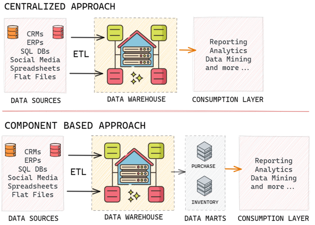
A simple end-to-end data warehousing environment consists of data sources, a data warehouse, and sometimes, smaller environments called data marts. The process connecting data sources to the data warehouse is known as ETL (Extract, Transform, and Load), a critical aspect of data warehousing.
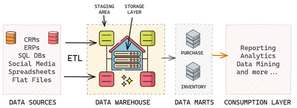
An analogy to understand this relationship is to think of data sources as suppliers, the data warehouse as a wholesaler that collects data from various suppliers, and data marts as data retailers. Data marts store specific subsets of data tailored for different user groups or business functions. Users typically access data from these data marts for their data-driven decision-making processes.
Data Warehouse Architecture
In data warehousing, there are various architectural options to plan and execute initiatives. These options include:
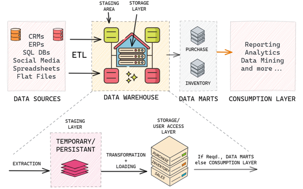
Staging layer: This is the segment within the data warehouse where data is initially loaded before it is transformed and fully integrated for reporting and analytical purposes. There are two types of staging layers: persistent and non-persistent.
Data marts: These are smaller-scale or more narrowly focused data warehouses.
Cube: A specialized type of database that can be part of the data warehousing environment.
Centralized data warehouse: This approach uses a single database to store data for business intelligence and analytics.
Component-based data warehousing: This approach consists of multiple components, such as data warehouses and data marts, that operate together to create an overall data warehousing environment.
Staging layer in a Data Warehouse
A data warehouse consists of two side-by-side layers: the staging layer and the user access layer. The staging layer serves as a landing zone for incoming data from source applications. The main objective is to quickly and non-intrusively copy the needed data from source applications into the data warehousing environment.
The user access layer is where users interact with the data warehouse or data mart. This layer deals with design, engineering, and dimensional modelling, such as star schema, snowflake schema, fact tables, and dimension tables.
There are two types of staging layers in a data warehouse: non-persistent staging layers and persistent staging layers. Both serve as landing zones for incoming data, which is then transformed, integrated, and loaded into the user access layer.
In a non-persistent staging layer, the data is temporary. After being loaded into the user access layer, the staging layer is emptied. This requires less storage space but makes it more difficult to rebuild the user layer or perform data quality assurance without accessing the original source systems.
In contrast, a persistent staging layer retains data even after it has been loaded into the user access layer. This enables easy rebuilding of the user layer and data quality assurance without accessing the source systems. However, it requires more storage space and can lead to ungoverned access by power users.
Data Warehouse vs Data Mart
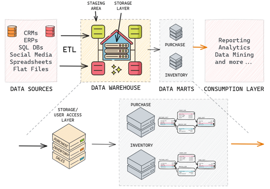
Data marts are additional environments in the data warehousing process, often thought of as data retailers. There are two
types of data marts: dependent and independent.
Dependent data marts rely on the existence of a data warehouse to be supplied with data. Independent data marts, on the
other hand, draw data directly from one or more source applications and do not require a data warehouse. Independent data
marts can be thought of as small-scale data warehouses with data organized internally.
The difference between a data warehouse and an independent data mart lies in the number of data sources and business
requirements. Data warehouses typically have many sources 1050, while independent data marts have much fewer data
sources. If a business requirement dictates the creation of well-defined business units due to the huge size of a data
warehouse, data marts can be added to the architecture to create units specific to business requirements such as purchase
specific data mart, inventory-specific data mart, etc. Other than that, the properties of a data warehouse and an independent
data mart are quite similar.
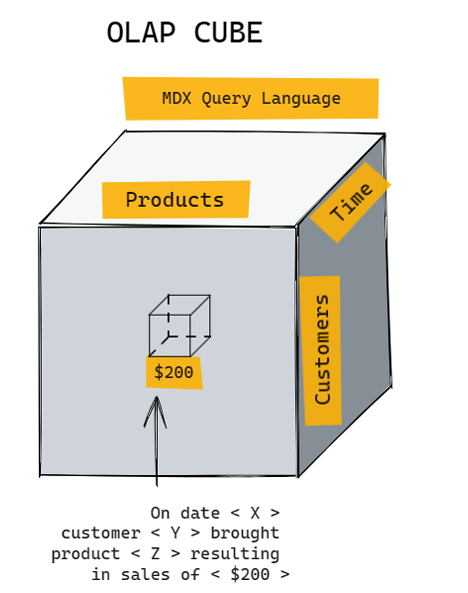
Cubes in Data Warehouse environment
Unlike relational database management systems RDBMS,
cubes are specialized databases with an inherent awareness
of the dimensionality of their data contents. Cubes offer
some advantages, such as fast query response times and
suitability for modest data volumes (around 100 GB or less).
However, they are less flexible compared to RDBMS, as they
have a rigid organizational structure for data. Structural
changes to the data can be complex and time-consuming.
Additionally, there is more vendor variation with cubes than
with RDBMS.
In modern data warehousing environments, it is common to
see a combination of relational databases and multi
dimensional databases. This mix-and-match approach can
provide a powerful combination for organizations.
Figuring out the appropriate approach to DW
In summary, there are two main paths to choose from when deciding on a data warehouse environment: a centralized
approach or a component-based approach.
A centralized approach, such as an Enterprise Data Warehouse EDW or a Data Lake, offers a single, unified environment for
data storage and analysis. This enables one-stop shopping for all data needs but requires a high degree of cross organizational cooperation and strong data governance. It also carries the risk of ripple effects when changes are made to the environment.
A component-based approach, on the other hand, divides the data environment into multiple components such as data
warehouses and data marts. This offers benefits like isolation from changes in other parts of the environment and the ability
to mix and match technology. However, it can lead to inconsistent data across components and difficulties in cross
integration.
The choice of data warehouse environment ultimately depends on the specific needs and realities of each organization, and
the decision-making process required.
Data Warehousing Design: Building
The primary objective of a data warehouse is to enable data-driven decisions, which can involve past, present, future, and
unknown aspects through different types of business intelligence and analytics. Dimensional modelling is particularly suited
for basic reporting and online analytical processing OLAP. However, if the data warehouse is primarily supporting predictive
or exploratory analytics, different data models may be required. In such cases, only some aspects of the data may be
structured dimensionally, while others will be built into forms suitable for those types of analytics.
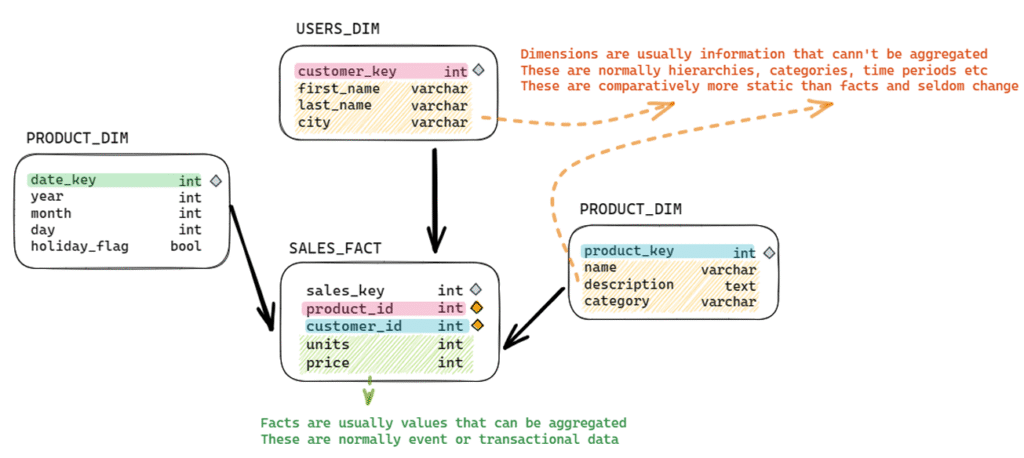
The Basic Principles of Dimensionality
Dimensionality in data warehousing refers to the organization of data in a structured way that facilitates efficient querying
and analysis. The two main components of dimensionality are facts/measurements and dimensional context, which are
essential for understanding the data and making data-driven decisions.
The main benefits of using a dimensional approach in data warehousing include:
Improved query performance By organizing data in a structured manner, queries can be executed more efficiently,
enabling faster data retrieval and analysis.
Simplified data analysis Dimensional models make it easier for analysts to understand the relationships between data
elements and perform complex analyses.
Enhanced data visualization Organized data enables better visualization of patterns, trends, and relationships, which in
turn helps in making informed decisions.
Facts/Measurements:
These are the quantifiable aspects of the data, such as sales amounts, user counts, or product quantities. They represent the
actual values or metrics that are being analyzed. It is important to differentiate between a data warehousing fact and a logical
fact, as the former is a numeric value while the latter is a statement that can be evaluated as true or false.
Fact tables store facts in a relational database used for a data warehouse. They are distinct from facts themselves, and there
are specific rules for determining which facts can be stored in the same fact table. Fact tables can be of different types and
can be connected with dimension tables to link measurements and context in the data warehouse.
Dimensional context:
This is the descriptive information that provides context to the measurements, helping to understand how the data is
organized and what it represents. Dimensions often include categories, hierarchies, or time periods, which enable data
analysts to slice and dice the data in various ways. Common dimensions include geography (e.g., country, region, city), time
(e.g., year, quarter, month), and product categories (e.g., electronics, clothing, food).
In a relational database, dimensions are stored in dimension tables. However, the terms “dimension” and “dimension table”
are sometimes used interchangeably, although they are technically different.
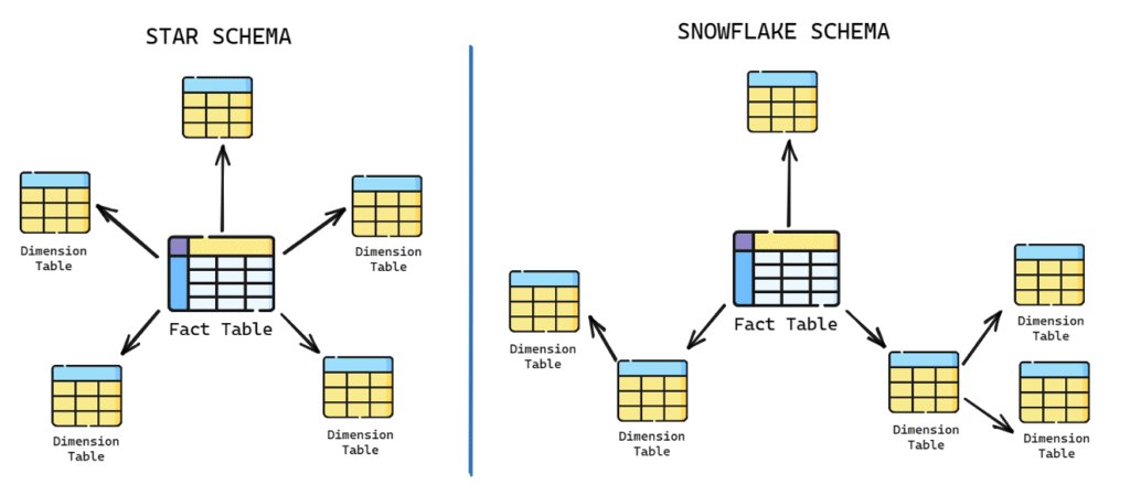
This interchangeability of terms is due to the differences between star and snowflake schemas. In a star schema, all
information about multiple levels of a hierarchy (e.g., product, product family, and product category) is stored in a single
dimension table, which is often called the product dimension table. In a snowflake schema, each level of the hierarchy is
stored in a separate table, resulting in three dimensions and three dimension tables.
Star schema and snowflake schema are two popular approaches to dimensional modelling. Both involve organizing data into
fact tables (which store measurements) and dimension tables (which store contextual information).
Star Schema vs Snowflake Schema
Star schema and snowflake schema are two different structural approaches to building dimensional models in a data
warehouse. Both are used to represent fact tables and dimension tables, which are essential for dimensional analysis in OLAP and business intelligence.
Comparison Between Star Schema and Snowflake Schema
| Feature | Star Schema | Snowflake Schema |
|---|---|---|
| Structure of Dimensions | All dimensions along a given hierarchy are stored in one dimension table. | Each dimension or sub-dimension is stored in its own separate table. |
| Distance from Fact Table | One level away from the fact table, requiring straightforward relationships. | One or more levels away from the fact table, requiring more complex relationships. |
| Database Joins | Fewer database joins required. | More database joins required. |
| Storage Requirement | Consumes more storage due to denormalized structure. | Consumes less storage due to normalized structure. |
Both star and snowflake schemas have the same number of dimensions, but their table representations differ. The choice
between star and snowflake schema depends on factors such as the complexity of the database relationships, storage
requirements, and the number of joins needed for data analysis.
Database Keys for Data Warehousing
Database keys play a crucial role in data warehousing. They help maintain relationships, ensure data integrity, and improve
query performance.
Primary Keys: A primary key is a unique identifier for each row in a database table. It can be a single column or a
combination of columns that guarantee the uniqueness of each record. Primary keys are essential for maintaining data
integrity, preventing duplicate entries, and providing a unique reference point for other tables.
Foreign Keys: A foreign key is a column or set of columns that reference the primary key of another table. The purpose of
foreign keys is to maintain the relationships between tables and ensure referential integrity. This means that a foreign key
value must always match an existing primary key value in the related table or be NULL. Foreign keys help with data
consistency, reduce redundancy, and make it easier to enforce constraints and retrieve related information.
Natural and Surrogate Keys
Natural Keys: Natural keys (also known as business keys or domain keys) are derived from the source system data and
are used to identify a record based on its inherent attributes. They can be cryptic or easily understandable, depending on
the nature of the data. Natural keys have their limitations, as they can be subject to change, and sometimes they may not
guarantee uniqueness. However, keeping natural keys in dimension tables as secondary keys can be beneficial for
traceability, data validation, and troubleshooting purposes.
For example, in a table storing employee details, the employee’s social security number could serve as a natural key.
Similarly, a customer’s email address could be a natural key in a customers table (assuming each customer has a unique
email address)
Surrogate Keys: Surrogate keys are system-generated, unique identifiers that have no business meaning. They are used
as primary keys in data warehousing to ensure data integrity and simplify the relationships between tables. Surrogate
keys are usually auto-incremented numbers. Surrogate keys are preferred over natural keys for several reasons, including
the ability to handle changes in the source data, improved performance, and the support for slowly changing dimensions.
For example, consider a table storing customer details. Even though each customer might have a unique email address, we might choose to use a surrogate key, such as CustomerID, to uniquely identify customers. So, a customer might be assigned an ID like 1, 2, 3, and so on, with no relation to the actual data about the customer.
Comparison:
Meaning Natural keys have a business meaning, while surrogate keys do not.
Change Natural keys can change (for example, a person might change their email address), while surrogate keys are
static and do not change once assigned.
Simplicity Natural keys can be complex if they’re composed of multiple attributes, while surrogate keys are simple
(usually just a number).
Performance Surrogate keys can improve query performance because they’re usually indexed and simpler to manage.
Data Anonymity Surrogate keys provide a level of abstraction and data protection, particularly useful when sharing data
without exposing sensitive information.
When designing a data warehouse, it is crucial to make the right choices regarding key usage. As a general guideline, use
surrogate keys as primary and foreign keys for better data integrity and handling of data changes. Keep natural keys in
dimension tables as secondary keys to maintain traceability and ease troubleshooting. Finally, discard or do not use natural
keys in fact tables, as they can lead to redundancy and complexity in managing the data warehouse.
Design Facts, Fact Tables, Dimensions, and Dimension Tables
Different Forms of Additivity in Facts
Additivity is an important concept in data warehousing that pertains to the rules for storing facts in fact tables. Facts can be
additive, non-additive, or semi-additive.
Additive facts can be added under all circumstances. For example, faculty members’ salaries or students’ credit hours can be
added together to find a total salary or total credit hours completed. These are valid uses of addition in the context of additive
facts.
Non-additive facts, on the other hand, cannot be added together to produce a valid result. Examples include grade point
averages GPA, ratios, or percentages. To handle non-additive facts, it’s best to store the underlying components in fact
tables rather than the ratio or average itself. You can store the non-additive fact at an individual row level for easy access but
should prevent users from adding them up. Instead, you can calculate aggregate averages or ratios from the totals of the underlying components.
Semi-additive facts fall somewhere between additive and non-additive facts, as they can sometimes be added together while at other times they cannot. Semi-additive facts are often used in periodic snapshot fact tables, which will be covered in more detail in future discussions.
NULLs in Facts
A NULL represents a missing or unknown value; Note that a Null does not represent a zero, a character string of one or more
blank spaces, or a “zero-lengthˮ character string.
The major drawback of Nulls is their adverse effect on mathematical operations. Any operation involving a Null evaluates to Null. This is logically reasonable—if a number is unknown, then the result of the operation is necessarily unknown
SELECT 5 + NULL; — Result: NULL
SELECT 10 – NULL; — Result: NULL
SELECT 3 * NULL; — Result: NULL
SELECT 15 / NULL; — Result: NULL
SELECT 8 % NULL; — Result: NULL– Assume a table ‘sales’ with a column ‘revenue’ containing the following values: –(10, NULL, 15)
SELECT SUM(revenue) FROM sales; — Result: 25 (ignores NULL values)
SELECT AVG(revenue) FROM sales; — Result: 12.5 (ignores NULL values)
SELECT COUNT(revenue) FROM sales; — Result: 2 (ignores NULL values)
SELECT COUNT(*) FROM sales; — Result: 3 (includes NULL values)
To handle NULL values in mathematical operations in MySQL, you can use functions like COALESCE or IFNULL to replace
NULL values with a default value. Here’s an example:– Replace NULL values with 0 and perform addition
SELECT 5 + COALESCE(NULL, 0); — Result: 5
SELECT 5 + IFNULL(NULL, 0); — Result: 5
NULLs also should be avoided in the foreign key column of fact tables. Instead of using NULLs, we can assign default values
to columns in the fact table. we can choose a value that represents the absence of data or a not applicable scenario.
However, even though this approach can simplify querying and analysis but it may introduce ambiguity if the default value
can be mistaken for actual data.
The Four Main Types of Data Warehousing Fact Tables
In data warehousing, there are four main types of fact tables used to store different types of facts or measurements.
Transaction Fact Table: This type of fact table records facts or measurements from transactions occurring in source
systems. It manages these transactions at an appropriate level of detail in the data warehouse.
Periodic Snapshot Fact Table: This table tracks specific measurements at regular intervals. It focuses on periodic
readings rather than lower-level transactions.
Accumulating Snapshot Fact Table: Similar to the periodic snapshot fact table, this table shows a snapshot at a point in
time. However, it is specifically used to track the progress of a well-defined business process through various stages.
Factless Fact Table: This type of fact table has two main uses. Firstly, it records the occurrence of a transaction even if
there are no measurements to record. Secondly, it is used to officially document coverage or eligibility relationships, even if nothing occurred as part of that particular relationship.
The Role of Transaction Fact Tables
Transactional fact tables are the most common type of fact table used in a data warehouse. These fact tables store
transaction-level data, meaning that each row in the table represents a single event or transaction. Transactional fact tables
are useful for capturing and analyzing detailed, granular data about the individual events that occur in a business. When
dealing with transaction fact tables, we can store multiple facts together in the same table if they meet the following rules:
Facts are available at the same grain or level of detail.
Facts occur simultaneously.
In a transactional fact table, each row is associated with one or more dimension tables. These dimension tables help provide
context and additional information about the transaction. Facts within the transactional fact table are usually numeric and
additive, such as sales amount, quantity sold, or total revenue.
Example:
Consider a retail store that wants to track sales transactions. In this example, the transactional fact table could be called
‘sales_fact’. For each sale transaction, the following information might be stored:
Date of sale Date Dimension)
Store location Store Dimension)
Product sold Product Dimension)
Customer information Customer Dimension)
Payment method Payment Method Dimension)
Quantity sold Fact)
Sales amount Fact)
Discount applied Fact)
Here is a simplified version of what the ‘sales_fact’ table might look like:
Sales Fact Table
| Transaction_ID (PK) | Date_Key (FK) | Store_Key (FK) | Product_Key (FK) | Customer_Key (FK) | Payment_Key (FK) | Quantity (Fact) | Sales_Amount (Fact) |
|---|---|---|---|---|---|---|---|
| 1 | 1 | 1 | 1 | 1 | 1 | 2 | 50 |
| 2 | 1 | 2 | 1 | 2 | 1 | 1 | 25 |
| 3 | 2 | 1 | 2 | 1 | 2 | 3 | 75 |
In this example, the transactional fact table contains three fact columns (quantity, sales_amount, and discount) and five
foreign key columns that connect to the respective dimension tables (date_key, store_key, product_key, customer_key, and
payment_key).
Remember to use surrogate keys (not natural keys) as primary and foreign keys to maintain relationships between tables.
These surrogate keys serve as foreign keys that point to primary keys in the respective dimension tables, which provide the
context needed for decision-making based on the data.
The Role of Periodic Snapshot Fact Tables
Periodic Snapshot fact tables are used in data warehouses to capture the state of a particular measure at specific points in
time, such as daily, weekly, or monthly snapshots. These fact tables help analyze trends and changes over time, which can be
valuable for understanding the business’s performance and making informed decisions.
In a periodic snapshot fact table, each row represents the state of a specific measure at a particular point in time. The table
typically includes one or more dimension keys that provide context for the snapshot, such as date, product, or customer
information.
Example:
Consider a bank that wants to track its customers’ account balances on a monthly basis. In this example, the periodic
snapshot fact table could be called ‘monthly_account_balance_fact’. For each customer, the following information might be
stored:
Snapshot Date Date Dimension)
Customer information Customer Dimension)
Account type Account Type Dimension)
Account balance Fact)
Here is a simplified version of what the ‘monthly_account_balance_fact’ table might look like:
Account Balance Snapshot Fact Table
| Snapshot_ID (PK) | Date_Key (FK) | Customer_Key (FK) | Account_Type_Key (FK) | Account_Balance (Fact) |
|---|---|---|---|---|
| 1 | 1 | 1 | 1 | 1000 |
| 2 | 1 | 2 | 1 | 2500 |
| 3 | 1 | 1 | 2 | 5000 |
| 4 | 2 | 1 | 1 | 1200 |
| 5 | 2 | 2 | 1 | 2300 |
| 6 | 2 | 1 | 2 | 5100 |
In this example, the periodic snapshot fact table contains one fact column (account_balance) and three foreign key columns
that connect to the respective dimension tables (date_key, customer_key, and account_type_key). Each row represents the
state of a customer’s account balance at the end of a specific month.
Using a periodic snapshot fact table, the bank can analyze its customers’ account balances in various ways, such as:
Average account balance per month
Changes in account balances over time
Distribution of account balances by account type
Customer segments based on account balances
Periodic snapshot fact tables are particularly useful for tracking and analyzing data that changes over time and may not be
easily captured in a transactional fact table. A complication with periodic snapshot fact tables is the presence of semi
additive facts.
Periodic Snapshots and Semi-Additive Facts
A semi-additive fact is a type of measure that can be aggregated along some (but not all) dimensions. Typically, semi-additive
facts are used in periodic snapshot fact tables.
The classic example of a semi-additive fact is a bank account balance. If you have daily snapshots of account balances, you
can’t add the balances across the time dimension because it wouldn’t make sense – adding Monday’s balance to Tuesday’s
balance doesn’t give you any meaningful information. However, you could add up these balances across the account
dimension (if you were to aggregate for a household with multiple accounts, for instance) or across a geographical dimension
(if you wanted to see total balances for a particular branch or region).
Here’s an example:
Daily Account Balance
| Date | AccountID | Balance |
|---|---|---|
| 2023-05-01 | 1 | 100 |
| 2023-05-01 | 2 | 200 |
| 2023-05-02 | 1 | 150 |
| 2023-05-02 | 2 | 120 |
| 2023-05-03 | 1 | 240 |
| 2023-05-03 | 2 | 250 |
If we were to add the balances across the time dimension (for example, to try to get a total balance for account 1 for the
period from May 1 to May 3, we would get $370, which doesn’t represent any meaningful quantity in this context. This is why
the balance is a semi-additive fact – it can be added across some dimensions (like the AccountID, but not across others (like
the Date).
In contrast, fully additive facts, like a bank deposit or withdrawal amount, can be summed along any dimension. Non-additive
facts, like an interest rate, cannot be meaningfully summed along any dimension.
When dealing with semi-additive facts, it’s important to ensure that your analysis is using the appropriate aggregation
methods for each dimension. Depending on the specific requirements of your analysis, you might need to use the maximum,
minimum, first, last, or average value of the semi-additive fact for a given period, rather than the sum.
The Role of Accumulating Snapshot Fact Tables
These tables are used to track the progress of a business process (e.g. order fulfillment) with formally defined stages,
measuring elapsed time spent in each stage or phase. They typically include both completed phases and phases that are in
progress. Accumulating snapshot fact tables also introduce the concept of multiple relationships from a fact table back to a
single dimension table.
These typically include multiple date columns representing different milestones in the life cycle of the event and one or more
dimension keys providing context for the snapshot, such as product, customer, or project information. The fact columns
represent the measures associated with each stage or milestone.
Example:
Consider a company that wants to track its sales orders from order placement to delivery. In this example, the accumulating
snapshot fact table could be called ‘sales_order_fact’. For each sales order, the following information might be stored:
Sales Order ID Primary key)
Customer information Customer Dimension)
Product Information Product Dimension)
Order date Date Dimension)
Shipping date Date Dimension)
Delivery date Date Dimension)
Order amount Fact)
Shipping cost Fact)
Here is a simplified version of what the ‘sales_order_fact’ table might look like:
Orders Fact Table
| Order_ID (PK) | Customer_Key (FK) | Product_Key (FK) | Order_Date_Key (FK) | Shipping_Date_Key (FK) | Delivery_Date_Key (FK) | Order_Amount (Fact) | Shipping_Cost (Fact) |
|---|---|---|---|---|---|---|---|
| 1 | 1 | 1 | 1 | 2 | 4 | 100 | 10 |
| 2 | 2 | 1 | 2 | 3 | 5 | 200 | 15 |
| 3 | 1 | 1 | 3 | 4 | 6 | 150 | 12 |
In this example, the accumulating snapshot fact table contains two fact columns (order_amount and shipping_cost) and five foreign key columns that connect to the respective dimension tables (customer_key, product_key, order_date_key, shipping_date_key, and delivery_date_key). Each row represents the life cycle of a sales order, from order placement to delivery.
Using an accumulating snapshot fact table, the company can analyze its sales order data in various ways, such as:
- Average time between order placement and shipping
- Average time between shipping and delivery
- Total shipping cost by product or customer
- Comparison of actual delivery dates to estimated delivery dates
In the accumulating snapshot fact table, there are multiple relationships with the same dimension table, such as the date dimension. This is because the table needs to track various dates related to the business process, like the order date, shipping date, delivery date, and so on. Similarly, multiple relationships with the employee dimension may also be required to account for different employees responsible for different phases of the process.
Comparing the three main types of fact tables
Comparison of Fact Table Types
| Feature | Transactional | Periodic Snapshot | Accumulating Snapshot |
|---|---|---|---|
| Grain | 1 row = 1 transaction | 1 row = 1 defined period (plus other dimensions) | 1 row = lifetime of process/event |
| Date Dimension | 1 transaction date | Snapshot date (end of period) | Multiple snapshot dates |
| Number of Dimensions | High | Low | Very High |
| Size | Largest (most detailed grain) | Middle (less detailed grain) | Lowest (highest aggregation) |
Why a Factless Fact Table isn’t a Contradiction in Terms
Fact tables are used in data warehouses to store facts or measurements that need to be tracked. A fact is different from a fact table, and there are various types of fact tables, each with a specific purpose and usage.
Factless fact tables are used in data warehousing to capture many-to-many relationships among dimensions. They are called “factless” because they have no measures or facts associated with transactions. Essentially, they contain only dimensional keys. It’s the structure and use of the table, not the presence of numeric measures, that makes a table a fact table.
Factless fact tables are used in two main scenarios:
1. Event Tracking In this case, the factless fact table records an event. For example, consider a table that records student attendance. The table might contain a student key, a date key, and a course key. There are no measures or facts in this table, only the keys of the students who attended classes on certain dates. The absence of facts is not a problem; simply capturing the occurrence of the event provides valuable information.
2. Coverage or Bridge Table This kind of factless fact table is used to model conditions or coverage data. For example, in a health insurance data warehouse, a factless fact table could be used to track eligibility. The table might contain keys for patient, policy, and date, and it would show which patients are covered by which policies on which dates.
Here’s an example of a factless fact table for an attendance system:
Student Course Enrollment
| Student_ID | Course_ID | Date (FK) |
|---|---|---|
| 1 | 101 | 2023-05-01 |
| 2 | 101 | 2023-05-01 |
| 1 | 102 | 2023-05-02 |
| 3 | 103 | 2023-05-02 |
This table does not contain any measures or facts. However, it provides valuable information about which student attended which course on which date. We can count the rows to know the number of attendances, join this with other tables to get more details, or even use this for many other analyses. The presence of a row in the factless fact table signifies that an event occurred.
Dimension Tables
Dimension tables in a data warehouse contain the descriptive attributes of the data, and they are used in conjunction with fact tables to provide a more complete view of the data. These tables are typically designed to have a denormalized structure for simplicity of data retrieval and efficiency in handling user queries, which is often essential in a business intelligence context.
Here are some key characteristics and components of dimension tables:
- Descriptive Attributes: These are the core of a dimension table. These attributes provide context and descriptive
characteristics of the dimensions. For example, in a “Customer” dimension table, attributes might include customer name,
address, phone number, email, etc. - Dimension Keys: These are unique identifiers for each record in the dimension table. These keys are used to link the fact
table to the corresponding dimension table. They can be either natural keys (e.g., a customer’s email address) or surrogate
keys (e.g., a system-generated customer ID. - Hierarchies: These are often present within dimensions, providing a way to aggregate data at different levels. For example,
a “Time” dimension might have a hierarchy like Year Quarter Month Day.
Example of a Dimension Table: Customer
Customer Dimension
| CustomerID (PK) | CustomerName | Gender | DateOfBirth | City | State | Country |
|---|---|---|---|---|---|---|
| 1 | John Doe | Male | 1980-01-20 | NY | NY | USA |
| 2 | Jane Smith | Female | 1990-07-15 | LA | CA | USA |
| 3 | Tom Brown | Male | 1985-10-30 | SF | CA | USA |
| 4 | Emma Davis | Female | 1995-05-25 | TX | TX | USA |
In this Customer dimension table, CustomerID is the surrogate key which uniquely identifies each customer. Other fields like CustomerName ,
Gender ,
DateOfBirth ,
City ,
State , and
Country provide descriptive attributes for the customers.
The “Sales” fact table in this data warehouse might then have a foreign key that links to the CustomerID in the dimension
table. This allows users to analyze sales data not just in terms of raw numbers, but also in terms of the customers.
In summary, dimension tables provide the “who, what, where, when, why, and how” context that surrounds the numerical
metrics stored in the fact tables of a data warehouse. They are essential for enabling users to perform meaningful analysis of
the data.