Learning Objectives
You will understand the available ingestion models in the bronze layers and the difference between them, and you will learn how the ingested data will be promoted to the silver layer.
When setting up ingestion into the bronze layer, we need to decide how input datasets should be mapped to the bronze tables.
Ingestion Patterns
We have two options: either
- Singleplex (1-to-1 mapping of source datasets to bronze tables)
- Multiplex (many-to-one mapping, meaning many datasets are mapped to one bronze table)
Singleplex
The singleplex is the traditional ingestion model where each data source or topic is ingested separately into a bronze table.
Here is an example of a bookstore dataset.
Each data source is ingested into a separate bronze table, so we end up here having three bronze tables, customers, books and orders.
These patterns usually work well for batch processing. However, for streaming processing of large datasets, if you have many streaming jobs, one per topic, you will hit the maximum limit of concurrent jobs in your workspace.
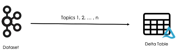
Multiplex
This combines many topics and stream them into a single bronze table.
In this model, we typically use a pub/sub system such as Kafka as a source, but we can also use files and cloud object storage with Auto Loader.
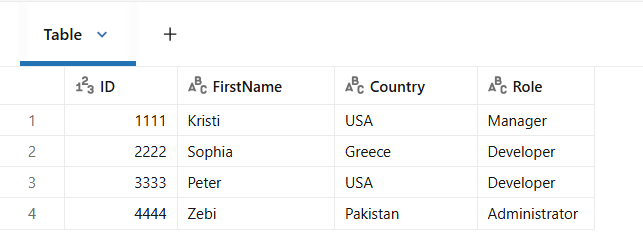
Coming back to our bookstore example, here we can see that all our input data has been ingested into a single bronze table.
In this table, records are organized into topics along with the value columns that contains the actual data in JSON format.
Later in the pipeline, the multiplex bronze table will be filtered based on the topic column to create the silver layer tables.
Practice
Let us now switch to Databricks workspace to see multiplex ingestion in action.
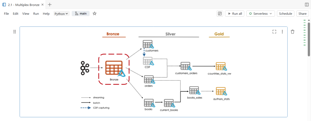
In this notebook, we are going to build a multiplex bronze table that store all topics of our bookstore dataset.
This single bronze table will drive the majority of data through the target architecture, feeding three independent data pipelines.
In this demonstration, rather than connecting directly to Kafka, our source system is going to send a row records as JSON files to cloud object storage.
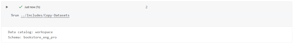
Let us start by copying our dataset files.
Before we start, let us explore our data source directory.
Currently we have one JSON file that contains raw Kafka data.
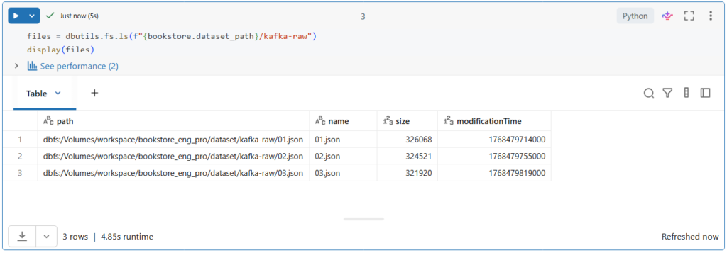
We will use Autoloader to read the current file in this directory and detect new files as they arrive in order to ingest them into the multiplex bronze table.
Let us take a look on this Kafka data.
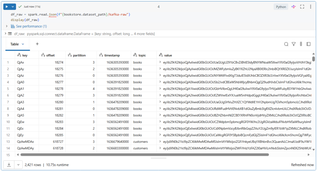
Here we see the full Kafka schema, including the topic, key and value columns that are encoded in binary.
This value column represents the actual data sent as JSON format.
In addition, we see the timestamp column representing the time at which the producer appended the records to a Kafka partition at a given offset.
Let us now write a function to incrementally process this data from the source directory to the bronze table.
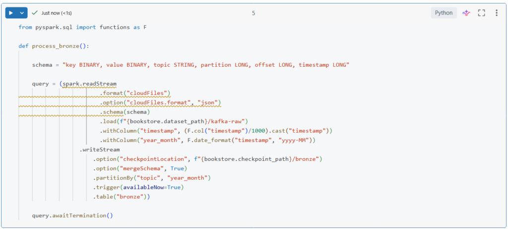
In this function, we start by configuring the stream to use Autoloader by specifying the cloudFiles format.
Then, we configure auto loader to use the JSON format and we provide the schema description.
Next, we parse the timestamp column from Unix timestamp into a human readable format.
And we extract year and month from this timestamp.
Lastly, we partition the table by the topic and the year_month fields.
.partitionBy("topic", "year_month")Depending on your data and business requirements, you can choose different columns for partitioning. For example, partitioning by week instead of month.
Notice here that we are using the merge schema option to leverage the schema evolution functionality of Autoloader.
.option("mergeSchema", True)This will automatically evolve the schema of the table when new fields are detected in the input JSON files.
Let us run this to create our function.
Now, let us call this function to process an incremental batch of data.

Since we are using the availableNow trigger option, our query executed in a batch mode.
.trigger(availableNow=True)It processed all the available data and then stopped on its own.
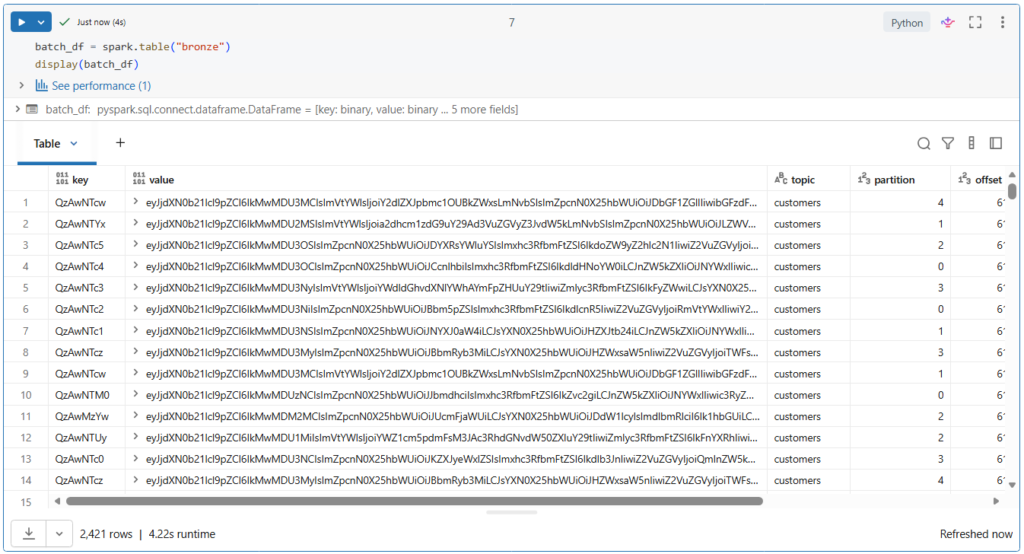
Let us review the data written to ensure records are being ingested correctly.
In Python, you can easily create a data frame from a registered table using the spark.table() function.
batch_df = spark.table("bronze")
display(batch_df)
Let us run this.
More than 2400 records have been ingested into our bronze table.
We can also use SQL to directly query the table.
SELECT * FROM bronze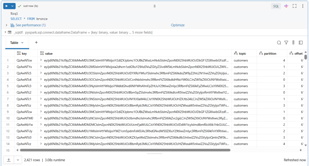
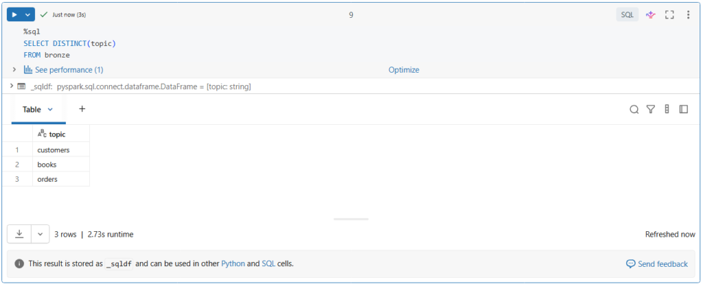
Let us list the topics ingested into our table.
SELECT DISTINCT(topic)
FROM bronze
As you can see, there are multiple topics in the bronze table.
Configuring Auto Loader for Reliable Ingestion
When using Auto Loader, you can configure several options for your stream to ensure reliable data ingestion:
Setting Maximum Bytes per Trigger
If you’re ingesting large files that cause long micro-batch processing times or memory issues, you can use the cloudFiles.maxBytesPerTrigger option to control the maximum amount of data processed in each micro-batch. This improves stability and keeps batch durations more predictable. For example, to limit each micro-batch to 1 GB of data, you can configure your stream as follows:
spark.readStream
.format("cloudFiles")
.option("cloudFiles.format", <source_format>)
.option("cloudFiles.maxBytesPerTrigger", "1g")
.load("/path/to/files")
Handling Bad Records
When working with JSON or CSV files, you can use the badRecordsPath option to capture and isolate invalid records in a separate location for further review. Records with malformed syntax (e.g., missing brackets, extra commas) or schema mismatches (e.g., data type errors, missing fields) are redirected to the specified path.
spark.readStream
.format("cloudFiles")
.option("cloudFiles.format", "json")
.option("badRecordsPath", "/path/to/quarantine")
.schema("id int, value double")     .load("/path/to/files")
Files Filters:
To filter input files based on a specific pattern, such as *.png, you can use the pathGlobFilter option. For example:
spark.readStream
.format("cloudFiles")
.option("cloudFiles.format", "binaryFile")
.option("pathGlobfilter", "*.png")
.load("/path/to/files")
Schema Evolution:
Auto Loader detects the addition of new columns in input files during processing. To control how this schema change is handled, you can set cloudFiles.schemaEvolutionMode option:
spark.readStream
.format("cloudFiles")
.option("cloudFiles.format", <source_format>)
.option("cloudFiles.schemaEvolutionMode", <mode>)
.load("/path/to/files")
The supported schema evolution modes include:

The default mode is addNewColumns, so when Auto Loader detects a new column, the stream stops with an UnknownFieldException. Before your stream throws this error, Auto Loader updates the schema location with the latest schema by merging new columns to the end of the schema. The next run of the stream executes successfully with the updated schema.
Note that the addNewColumns mode is the default when a schema is not provided, but none is the default when you provide a schema. addNewColumns is not allowed when the schema of the stream is provided.